First Principles

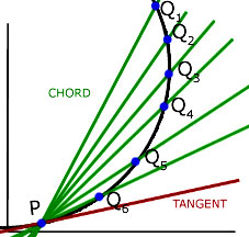
To find an expression for the gradient of the tangent at point P on a curve, we must consider lines passing through P and cutting the curve at points Q₁ Q₂ Q₃ Q₄ Q₅ Q₆ ...etc.

As Q approaches P so the gradient of the chord PQ approaches the gradient of the tangent at P.

We can form an expression for the gradient at P by using this concept.

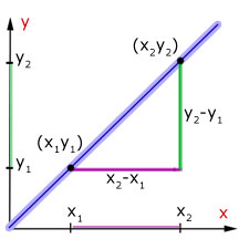
We know from coordinate geometry that:

Consider the coordinates of P to be (x,y) and point Q to be(x+dx, y+dy), where dx and dy are the horizontal and vertical components of the line PQ.

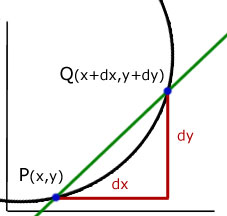
Gradient of the line between points (x,y) and (x+dx, y+dy) is given by :

The tangent to the curve = gradient of PQ when the length of PQ is zero and dx = 0 and dy = 0.

in the limit, as dx 'approaches zero' the gradient of the curve is said to be dy/dx.

If we now replace y by f(x) in the expression for gradient, since y = f(x) i.e. y is a function of x.

and

y = f(x)

y + dy = f(x + dx)

we have:

that is,

Example: find the gradient of y = 4x²

cancelling by dx

in the limit when dx = 0 this becomes,

Without doubt this is a very long winded way to work out gradients. There is a simpler way, by using the Derivative Formula.

Notation This is best described with an example.

If y = 3x² , which can also be expressed as f(x)= 3x², then

the derivative of y with respect to x can be expressed as:

The Derivation Formula

If we have a function of the type y = k xⁿ , where k is a

constant, then,

example #1

Find the gradient to the curve y = 5 x² at the point (2,1).

gradient = (5) (2 x^2-1) = 10 x¹ = 10 x

gradient at point (2,1) is 10 x 2 = 20

Differentiation Calculus Formulas:

1. $\displaystyle\frac{{d}}{{\left.{d}{x}\right.}}$ (xⁿ) = n x^n-1

2. $\displaystyle\frac{{d}}{{\left.{d}{x}\right.}}$ (ln x) = $\displaystyle\frac{{1}}{{x}}$

3. $\displaystyle\frac{{d}}{{\left.{d}{x}\right.}}$ (cos x) = −sin x

4. $\displaystyle\frac{{d}}{{\left.{d}{x}\right.}}$ (e^x) = e^x

5. $\displaystyle\frac{{d}}{{\left.{d}{x}\right.}}$ (tan x) = sec²x

6. $\displaystyle\frac{{d}}{{\left.{d}{x}\right.}}$ (sin x) = cos x

7. $\displaystyle\frac{{d}}{{\left.{d}{x}\right.}}$ (log_b u) = $\displaystyle\frac{{1}}{{{u}{\ln{{b}}}}}$ $\displaystyle\frac{{{d}{u}}}{{{\left.{d}{x}\right.}}}$

8. . $\displaystyle\frac{{d}}{{\left.{d}{x}\right.}}$ $\displaystyle{\left(\frac{{u}}{{v}}\right)}$ = $\displaystyle\frac{{{v}\frac{{{d}{u}}}{{{\left.{d}{x}\right.}}}-{u}\frac{{{d}{v}}}{{{\left.{d}{x}\right.}}}}}{{{v}}^{{2}}}$

9. $\displaystyle\frac{{d}}{{\left.{d}{x}\right.}}$ $\displaystyle{\left({u}{v}\right)}$ = $\displaystyle{u}\frac{{{d}{v}}}{{{\left.{d}{x}\right.}}}$ + $\displaystyle{v}\frac{{{d}{u}}}{{{\left.{d}{x}\right.}}}$

Learning Differentiation Online Study Problems:

Learning differentiation online study Problem 1:

Solve the differentiation logarithmic function f(x) = ln(4x + 10) with respect to x.

Solution:

Let u = 4x + 10 So, f(x) = ln u

$\displaystyle\frac{{{d}{u}}}{{{\left.{d}{x}\right.}}}$ = 4

f(x) = ln u

$\displaystyle\frac{{d}}{{\left.{d}{x}\right.}}$ (f(x)) = $\displaystyle\frac{{d}}{{\left.{d}{x}\right.}}$ ( ln u) we know, $\displaystyle\frac{{d}}{{\left.{d}{x}\right.}}$ (ln u) = $\displaystyle\frac{{1}}{{u}}$ $\displaystyle\frac{{{d}{u}}}{{{\left.{d}{x}\right.}}}$

= $\displaystyle\frac{{1}}{{u}}$ $\displaystyle\frac{{{d}{u}}}{{{\left.{d}{x}\right.}}}$

= $\displaystyle\frac{{1}}{{{4}{x}+{10}}}{\left({4}\right)}$

= $\displaystyle\frac{{4}}{{{4}{x}+{10}}}$

Answer: Differentiation of ln(4x + 10) is $\displaystyle\frac{{4}}{{{4}{x}+{10}}}$

Learning differentiation online study Problem 2:

Solve the differentiation of given function y = x³ - 7cot x.

Solution:

Let y = x³ - 7cot x

$\displaystyle\frac{{{\left.{d}{y}\right.}}}{{\left.{d}{x}\right.}}$ = $\displaystyle\frac{{d}}{{\left.{d}{x}\right.}}$ [x³ - 7cot x]

= 3x² $\displaystyle\frac{{{\left.{d}{x}\right.}}}{{\left.{d}{x}\right.}}$ - 7 $\displaystyle\frac{{d}}{{\left.{d}{x}\right.}}$ (cot x) (we know . $\displaystyle\frac{{d}}{{\left.{d}{x}\right.}}$ (cot x) = - cosec²x)

= 3x² - 7(-cosec²x)

= 3x² + 7cosec²x

Answer: Differentiation of x³ - 7cot x is 3x² + 7cosec²x

Learning differentiation online study Problem 3:

Solve the differentiation of exponential function 10e^4x

Solution:

$\displaystyle\frac{{d}}{{\left.{d}{x}\right.}}$ (10e^4x) = 10 $\displaystyle\frac{{d}}{{\left.{d}{x}\right.}}$ e^4x

Here, a = 4

So, = 10 $\displaystyle\frac{{d}}{{\left.{d}{x}\right.}}$ e^4x

= 10(4) e^4x

= 40 e^4x

Answer: Differentiation of 10e^4x is 40 e^4x

Differential Calculus Formulas

If you can't view the formulas correctly, then you need to download FireFox Web Browser.

Rules

Sum Rule:
${[f (x) \pm g (x)]}^{'}$ = f′(x) ± g′(x)
Product Rule:
${[f (x) \cdot g (x)]}^{'}$ = f′(x) · g(x) + f(x) · g′(x)
Quotient Rule:
${[f (x)}^{g (x)]'}$ = f′(x) · g(x) − f(x) · g′(x) g2(x)
Chain Rule:
${[f \circ g (x)]}^{'}$ = f′(g(x)) · g′(x)
Inverse Rule:
$[$ f − 1 ] ′ ( t ) = 1 f ′ ( f − 1 ( t ) )

Reference Formulas:

$d$ dx c = 0
$d$ dx c f ( x ) = c d dx f ( x )
$d$ dx x n = n x n − 1
$d$ dx sinax = acosax
$d$ dx cosax = −asinax
$d$ dx tan x = sec 2 x
$d$ dx cot x = − csc 2 x
$d$ dx sec x = sec x tan x
$d$ dx csc x = − csc x cot x
$d$ dx e a x = a e x
$d$ dx a x = ln ( a ) a x , a > 0 & a ≠ 1
$d$ dx ln x = 1 x
$d$ dx log a ( x ) = 1 ln ( a ) x , a > 0 & a ≠ 1
$d$ d x arcsin x = 1 1 − x 2
$d$ d x arccos x = − 1 1 − x 2
$d$ d x arctan x = 1 1 + x 2

Differential and Integral Calculus

1. Hyperbolic Functions

2. Convergence of Sequences and Series

2.1 Infinite sequences

Cauchy's convergence test

A sequence of numbers a_nis convergent if, and only if, there exists for every positive constant e a number N such that

Operating with limits

exist, then

2.2 Infinite Series 8:

Cauchy's convergence test

The series Sa_nconverges if, and only if, for there exists for every positive quantity e a number N such that

Note: All the following criteria are sufficient, but not necessary.

Principal of Comparison of Series 8.2 Sa_n converges if there exist numbers b_nsuch that b_n³ |a_n| for all values of n and Sb_nconverges.

Ratio test and and root test

Sa_nconverges if there is a number N, and also a number q < 1 such that

for all values n > N; in particular, if there is a number k < 1 such that

Leibnitz's Test

Sa_n converges if the terms have alternating signs and |a_n| tends monotonically to zero.

3. Differentiation

3.1 General rule (Fundamental Ideas:

Chain Rule

with corresponding formulae for u_xy and u_yy

Implicit Functions

Functions expressed in terms of a parameter

Inverse functions

3.2 Special Formulae

4. Integration

4.1 General Rules (Fundamental Ideas)

Estimation of Integrals

Integration by Parts

Method of Substitution

Link between Differentiation and Integration

Improper Integrals

If f(x) is continuous except at the point x = b, where it becomes infinite, is (absolutely) convergent, if in the neighbourhood of x = b

where n > 1, for values of x ³ A.

4.2 Special Formulae

Recurrence Relations

4.3 Integration of Special Functions

4.3.1 Rational functions

These are reduced to the following three fundamental types by resolution into partial fractions

the integral on the right hand side being evaluated by the last recurrence relation above;

where the integral on the right hand side is of the preceding type.

In the sequel, R denotes a rational function.

Substitution: t = tan x/2, so that

However, if R is an even function or only involves tan x, the following substitution is more convenient:

Substitution t = tanh x/2, so that

Substitution t = e^mx, dx/dt = 1/mt.

Substitution:

The substitution reduces this integral to one of the preceding three types.

Substitution:

5. Uniform Convergence and Interchange of Infinite operations

For the definition of uniform convergence go to

A series, which is uniformly convergent in a closed interval and the terms of which are continuous functions, represents a continuous function in the interval

If |f(x)| £ a_nand Sa_nconverges, Sf_n(x) converges uniformly ( and absolutely).

Interchange of summation and differentiation

Any convergent series of continuous functions may be differentiated term by term, provided the resulting series converges uniformly.

Interchange of summation and integration

Any uniformly convergent series of continuous functions may be integrated term by term. The resulting series also converges uniformly.

6. Special Links

Stirling's Formula

Wallis' Product

Infinite products

Definition of the Gamma function

if x is a positive integer n,

Order of magnitude of functions

7. Special Definite integrals

Orthogonality relations of the trigonometric functions

8. Mean Value theorem

Mean value theorem of the differential calculus

If f(x) = f(x + h) = 0, this yields Rolle's theorem : Between two zeros of the function lies always a zero of the derivative.

Generalized Mean Value theorem

where x is a value between a and b.

Taylor's theorem

with the remainder

Mean value theorem of the integral calculus

9. Expansion in Series: Taylor Series, Fourier Series

1. Power series Definition

9.1.1 Power series in general

Any power series

in one variable has a radius of convergence r (which may be zero or infinite); the series converges when |x| < r; in fact, it converges uniformly and absolutely in every interval |x| £h, where h < r; when |x| > r; the series diverges

If the remainder in Taylor's theorem tends to zero as n increases, we have the infinite power series

9.1.2 Special Taylor series

where the B_nare Bernoulli numbers A8.4.

9.1.3 Binomial series

9.1.4 Elliptic integral

9.2 Fourier series

If the function f(x) is sectionally smoot

h in the interval -p £ x £ p, i.e., if its first derivative is sectionally continuous, the Fourier series

is absolutely convergent throughout the entire interval. If f(x) has a finite number of jump discontinuities, while f '(x) is elsewhere sectionally continuous, the series converges uniformly in every closed subinterval which contains no discontinuities of f(x). At every point at which f(x) is continuous, the series represents the value of the function f(x), while at every point of discontinuity of f(x) it represents the arithmetic mean of the right hand and left hand limits of f(x).

10. Maxima and Minima

The following rule holds only for maxima and minima in the interior of the region under consideration.

In order that x may be an extreme value of the function y = f(x), f '(x) must vanish. When this condition is satisfied, there is a maximum or minimum, if the first non-vanishing derivative of f(x) is of even order; if it is of odd order, there is neither a maximum nor a minimum. In the former case, there is a maximum or a minimum according to whether the sign of the first non-zero derivative is negative or positive .